Ontology RAG Guide
Extract structured data using schemas and ontologies to define relationships and types using the Workbench
Intermediate
15 min
- TrustGraph deployed (Installation Guide)
- Understanding of Core Concepts
- Familiarity with ontologies and schemas
Import OWL ontologies, extract structured knowledge using schemas, and query ontology-based knowledge graphs.
Extract knowledge using language definition
Ontology RAG is a technique which uses automated extraction of relationships from unstructured text, which is stored in a knowledge graph. It is similar to GraphRAG.
Ontology RAG uses an ontology, which is a form of schema, defining the semantic meaning of language concepts.
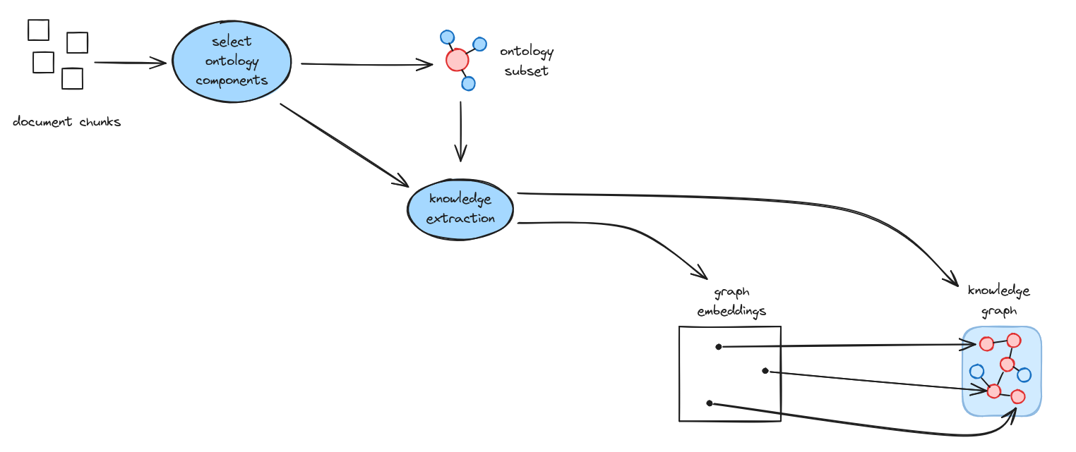
In TrustGraph, Ontology RAG refers to information extraction using an ontology. TrustGraph supports importing OWL ontologies which can then be used to import objects and properties from unstructured text.
What is Ontology RAG?
The essential Graph RAG ingest flow consists of:
- Chunking documents into smaller pieces
- Ontology loading an OWL ontology is loaded into an in-memory store
- Knowledge Extraction using the ontologies to discover entities and relationships
- Embedding each entity as a vector and storing these in a vector store
- Storing entity relationships in a knowledge graph
- Retrieving using semantic similarity to discover knowledge graph entry points
- Traversing the knowledge graph to find related information
- Generating responses using the knowledge subgraph as context to an LLM
The pros and cons of this approach:
- ✅ Pro: Very precise retrieval
- ✅ Pro: Conformant knowledge graphs - knowledge graph structures are defined by the ontologies
- ✅ Pro: Effective when faced with complex relationships or diverse data
- ✅ Pro: Scales to handle much larger document sets and complex ontologies
- ⚠️ Con: Knowledge extract has a cost at document ingest time
- ⚠️ Con: Token costs required to ingest documents
- ⚠️ Con: Ontology creation can be a complex process
When to Use Ontology RAG
✅ Use Ontology RAG when:
- Ontologies already exist for your information space
- Answers need context from multiple documents
- You need to connect disparate information
- Complex custom knowledge problems require precision of retrieval
- Working with specialist knowledge such as cybersecurity or intelligence
⚠️ Consider alternatives when:
- Simple keyword search on small data is sufficient → Use Document RAG
- Ontology defintion will be too complex → Use GraphRAG
Prerequisites
Before starting:
- ✅ TrustGraph deployed (Installation Guide)
- ✅ Understanding of Core Concepts)
Step-by-Step Guide
Step 1: Load the Ontology
The ontology we’re going to use is the SSN with SOSA extensions. This is a standard ontology family defined by the W3C.
SOSA (Sensor, Observation, Sample, and Actuator) and SSN (Semantic Sensor Network) are standardized vocabularies for describing sensors, observations, and measurements on the web. They’re maintained by the W3C (World Wide Web Consortium).
Think of them as a shared language that lets different systems talk about sensor data in a consistent way.
The Relationship Between Them
SOSA is the lightweight core — it defines the essential concepts you need to describe observations and sensors. SSN builds on top of SOSA, adding more detailed concepts for complex scenarios.
You can use SOSA alone for simple cases, or bring in SSN when you need more expressive power.
Core Concepts in SOSA
The main classes you’ll work with are:
- Sensor - A device or agent that observes something (a thermometer, a satellite, even a human observer).
- Observation - The act of measuring or estimating a property. An observation links together what was observed, how it was observed, and what the result was.
- ObservableProperty - The quality being measured (temperature, humidity, speed).
- FeatureOfInterest - The real-world thing you’re interested in (a room, a lake, a patient).
- Result - The output value of an observation.
- Actuator and Actuation - The counterparts for doing something rather than observing (turning on a heater, opening a valve).
- Sample - A representative portion of a larger feature (a water sample from a lake).
A Simple Example
Imagine a weather station measuring air temperature:
- FeatureOfInterest: The atmosphere at a specific location
- ObservableProperty: Air temperature
- Sensor: A digital thermometer
- Observation: The act of taking a reading at 2pm on Tuesday
- Result: 22.5 degrees Celsius
How TrustGraph uses ontologies
TrustGraph stores ontologies as an internal JSON format which is not standard but closely follows the OWL Ontology structure.
You can create an ontology using the Workbench Ontology editor. This is able to import a standard OWL ontology.
Download the ontology in standard Turtle format at the following URL:
Then load the ontology:
- On the Workflows page, select Ontology Management
- Click Import OWL/Turtle… at the bottom of the panel
- Select the ontology file you just downloaded
At this point you should be looking at a structured view of the ontology. The ontology editor can be used to explore and add information to an existing ontology. The ontology contains classes, properties and datatypes.
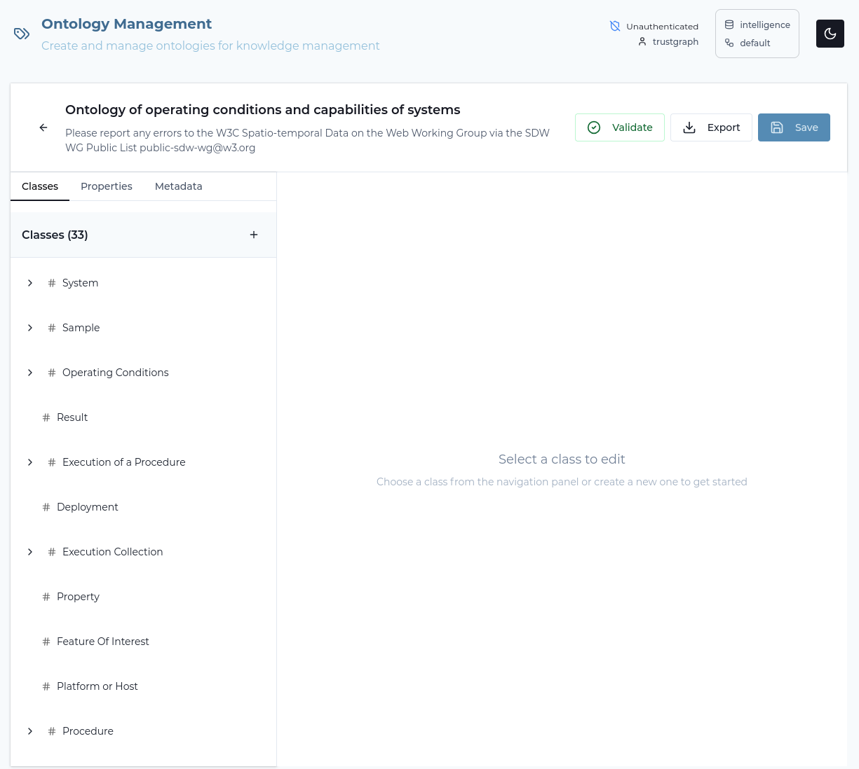
OWL (Web Ontology Language) ontologies are formal descriptions of concepts and their relationships within a domain. They define classes (types of things), properties (relationships between things), and constraints on how those relate. A full treatment of OWL ontologies is beyond the scope of this guide.
If you want to create your own ontologies, your favourite LLM (e.g. Claude or Gemini) can help move from a discussion of the information space to drafting OWL ontologies. Make sure to capture them in Turtle format, and tell the LLM to use rdfs:label and rdf:description on all ontology elements — this is needed to power TrustGraph’s ontology extraction pipeline.
Step 2: Load Your Document
TrustGraph supports multiple document formats:
- PDF files (
.pdf) - Text files (
.txt) - Markdown (
.md) - HTML (
.html)
We’re going to start by using a fictional maritime tracking report which you can download at this URL:
- Download the document
- Go to the Workflows page and click + Add Document
- A new dialogue appears — click the filename button and select the file you downloaded. The MIME type field should fill in automatically.
- Set the Title: Operation PHANTOM CARGO
- Set the Description to: Intelligence report: Operation PHANTOM CARGO
- Add tags: phantom cargo, intelligence, maritime, shipping
- Click Upload
The document shows upload progress. On upload completing, the new document outline changes to a solid line.
Step 3: Submit the Document for Processing
Once the document is uploaded, click Submit for Processing on the document detail panel. A 3-step wizard appears to select a flow and collection.
Select a flow: For Ontology RAG we need to start a new flow. The wizard shows available flow blueprints:
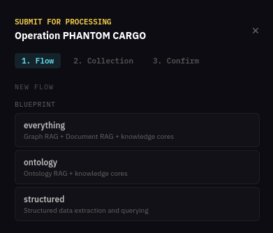
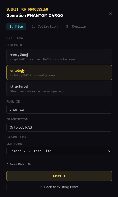
Select the ontology blueprint. Set the Flow ID to onto-rag and the Description to Ontology RAG. You can also select the LLM model to use and adjust advanced parameters.
Select a collection: Choose which collection the results should be stored in. For this guide, select default.
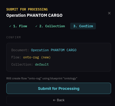
Confirm: Review the document, flow and collection selections. Note that it shows the new flow will be created using the ontology blueprint. Click Submit for Processing.
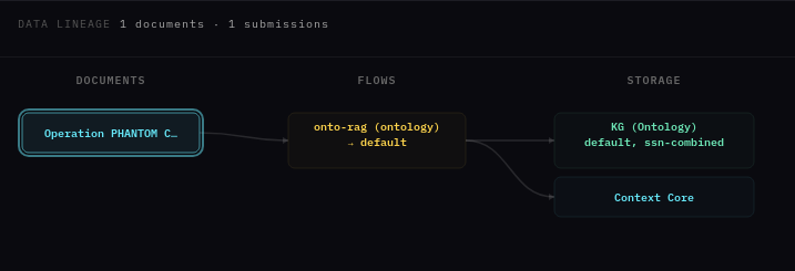
The main page reconfigures to show the document with its processing pipelines. Note that Ontology RAG produces a KG (Ontology) store and a Context Core — unlike the default flow, there is no Chunk Store because Ontology RAG does not run Document RAG processing.
Step 6: Monitoring
If you want to see the document loading, you can go to Grafana at http://localhost:3000. Login with username admin and the password you set in GF_SECURITY_ADMIN_PASSWORD. Grafana is configured with a single dashboard. Some useful things to monitor are:
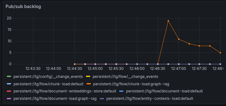
The pub/sub backlog. You can monitor the size of queues in Pulsar. Knowledge extraction causes a queue of chunks for processing in knowledge extraction and you can see this in the backlog:
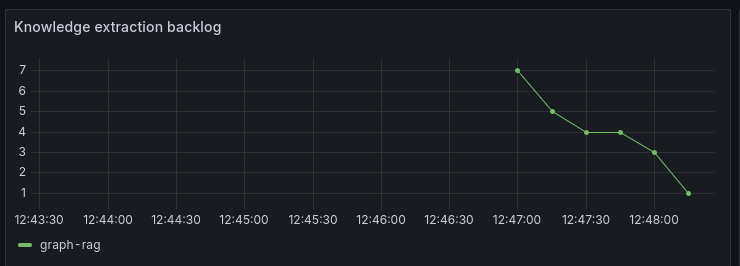
There is also a knowledge extraction backlog graph which helps to see knowledge extraction if other queues are being exercised:
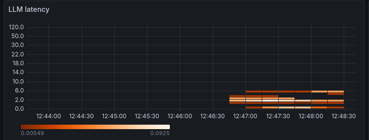
To gauge LLM effectiveness, there is a heatmap which shows LLM latency. Here we can see that LLM response times for my LLM processing are in the 6 second window.
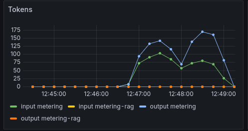
Another LLM effectiveness graph, the Token graph shows token throughput over time, the Y-axis shows tokens/s rate.
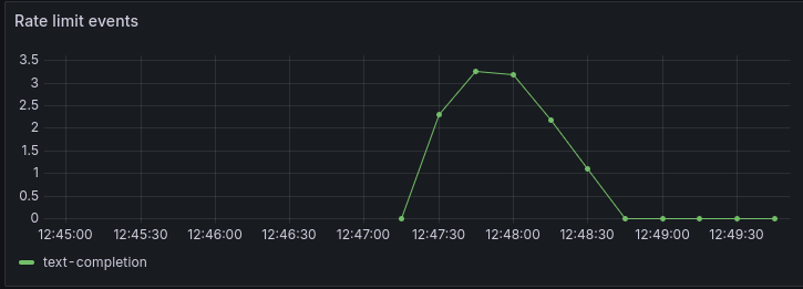
Finally, another useful chart shows the rate limit events per second. These are commonly seen in the text-completion process which interfaces with the LLM. Rate limit events are normal for a knowledge extraction backlog. This might particularly be helpful for you to determine whether you need to provision more LLM bandwidth or dedicated hosting.
The document we loaded is small, and will process very quickly, so you should only see a ‘blip’ on the backlog showing that chunks were loaded and cleared quickly.
It can take many minutes or hours to process large documents or large document sets using Ontology RAG extraction.
Step 7: Context Graph
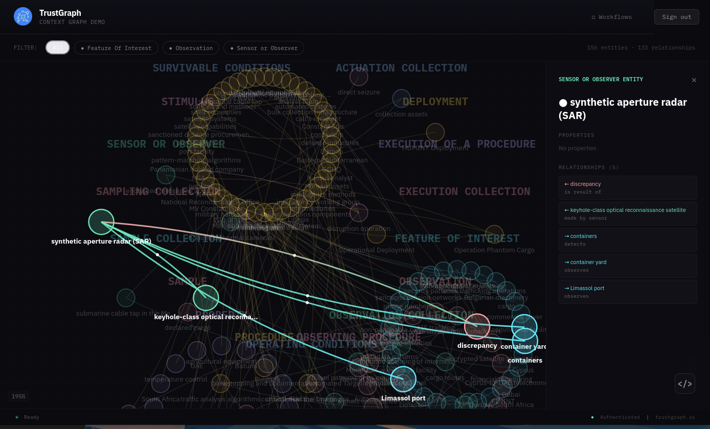
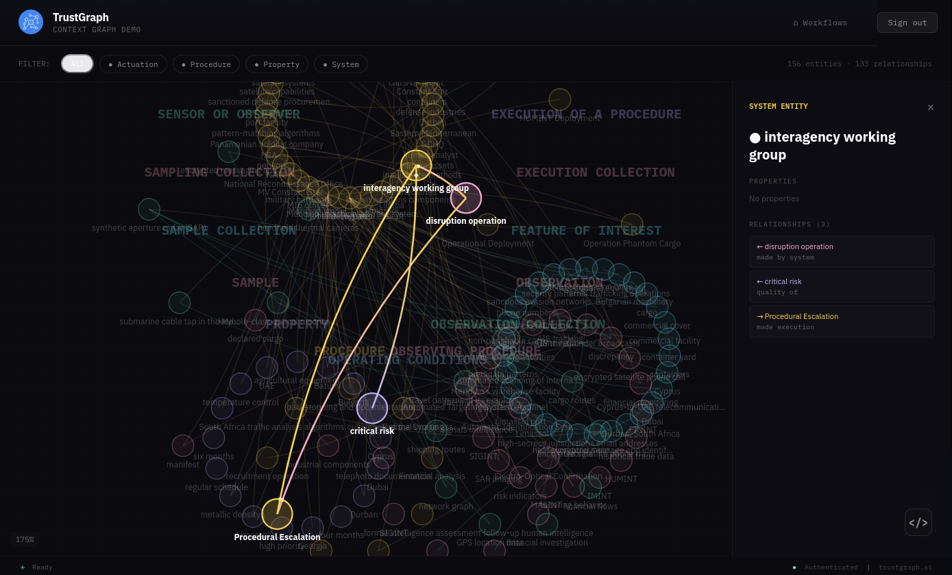
From the Workflows page, select Context Graph. This is similar to the Graph Explorer but takes advantage of the richer type information in an ontology-based knowledge graph by clustering nodes around their ontology types. Because the graph has much more type information, the Context Graph provides a powerful way to visualise and navigate the structured knowledge.
Clicking a node highlights it and its related edges, and opens a detail panel on the right showing node properties and navigation links.
Ontology Viewer
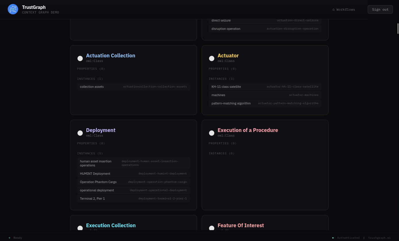
From the Workflows page, select Ontology Viewer. This displays the ontology types as cards with their extracted instances listed beneath them. This is another way to explore the ontology-based knowledge graph, showing how extracted entities have been classified against the ontology types.
Note that this view relies on ontology processing having completed — it is not enough to have loaded an ontology. Without ontology processing there will be no instances to display.
Step 8: Query with Graph RAG
From the Workflows page, select Graph RAG Query. This console has full Explainable AI enabled, which helps to understand and diagnose retrieval.
Enter the question: What intelligence resources were using during the PHANTOM CARGO operation? After a short while you should see a response.
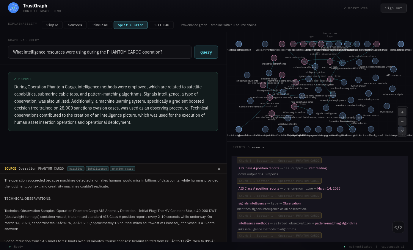
On the left-hand side you see the answer to the query. The bottom right part of the screen shows the various explainability events, starting from the question:
- Grounding — where retrieval selects key concepts for discovery
- Exploration — where graph nodes are selected for analytics
- Focus — where the system decides on a core set of graph edges to resolve the question
- Synthesis — where this is processed to provide an answer
The Focus event may be of particular interest as you can trace graph edges all the way back to the source documents.
Step 9: Explore the knowledge graph
From the Workflows page, select Graph Explorer. This shows what’s in the knowledge graph with tools for viewing and searching.
The graph can be easier to see in 3D — click the 3D button above the graph view.
If you click a node, it will be highlighted along with its related edges. A side panel also appears showing node properties and highlighted links that allow you to navigate to related nodes.
On the top left is a Search button which opens a search dialog. You can enter text for a similarity search against nodes in the graph. Matching nodes are listed and can be selected, which adds them to the graph along with their neighbours.
Ontology RAG provides a much richer set of connections in the graph compared to schema-free Graph RAG, so expect to see more consistency and more inter-connected paths in the knowledge graph explorer.
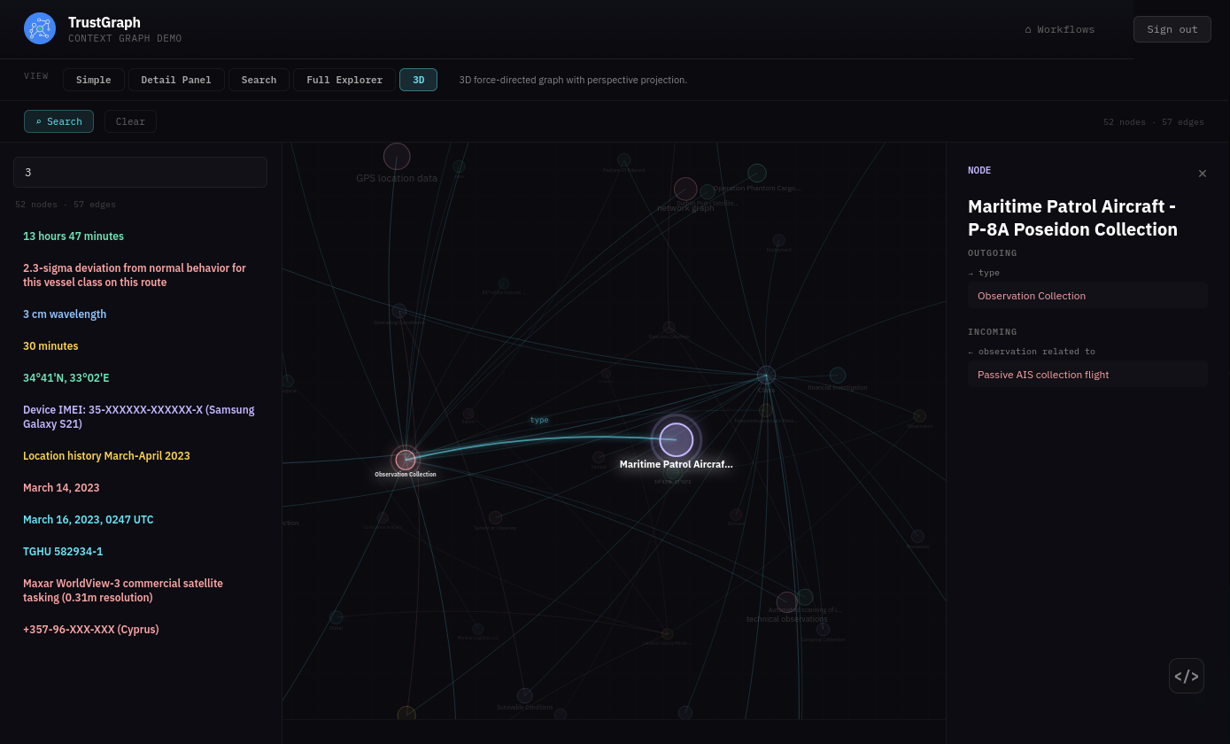
There is also a Clear button which resets the graph back to an empty state.
Further exploration
If you want to try a RAG approach but don’t know where to start, an interesting experiment is to compare GraphRAG and Ontology RAG to see which works best for your use-case.
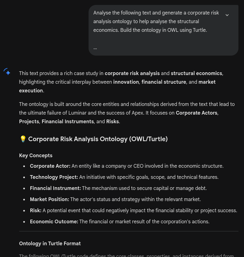
If you don’t know anything about ontologies, you could try using Claude to generate an ontology. Feed in some text, tell the assistant the important use-cases and ask for an OWL ontology presented in Turtle format.
Conclusion
The advantage of Ontology RAG is that it guides the knowledge extraction to extract knowledge in a particularly precise manner. For complex use-cases this means that the knowledge going into retrieval contexts is packed with the right information to answer the question. This is a major advantage for complex information analysis use-cases.
Ontology RAG vs. Other Approaches
| Aspect | Document RAG | Graph RAG | Ontology RAG |
|---|---|---|---|
| Retrieval | Vector similarity | Graph relationships | Schema-based |
| Context | Isolated chunks | Connected entities | Connected objects, properties and types |
| Best for | Semantic search | Complex relationships | Complex relationships + precise types |
| Setup | Simple | Simple | Complex |
| Speed | Fast | Medium | Medium |
Use multiple approaches: The processing flow defines the extraction and retrieval mechanisms, so you can use multiple approaches on the same data.
Next Steps
Explore Other RAG Types
- GraphRAG - Schema-free automated knowledge extraction
Advanced Features
- Structured Processing - Extract typed objects
- Agent Extraction - AI-powered extraction workflows
- Object Extraction - Domain-specific extraction
Using the CLI
For command-line workflows, see the Ontology RAG CLI Guide.
Related Resources
- Graph RAG - Schema-free knowledge extraction
- Working with Context Cores - Package and share knowledge
- Getting Started - Introduction to TrustGraph